3 Riemannian Geometry

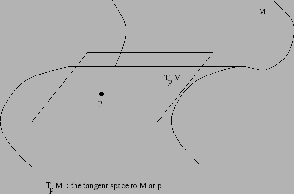
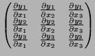
Let us now consider a small region M of space on which it is possible to put coordinates, say (x₁, x₂, x₃). Moreover, any other choice of coordinates, say (y₁, y₂, y₃) is differentiable (to any order) with respect to the given choice, that is to say the y_i are differentiable functions of the x_i, and vice versa. Then we have the non-singularity of the Jacobian matrix

J(y, x) = $$\begin{pmatrix} \frac{\partial y_1}{\partial x_1} & \frac{\parti... ...{\partial y_3}{\partial x_2} & \frac{\partial y_3}{\partial x_3} \end{pmatrix}$$.

The basic geometric notion other than that of points of the space is the notion of tangent vectors at points. At any point these represent the physical notion of instantaneous velocities and form a linear space of dimension 3 called the tangent space at the given point. In some sense this space is the Euclidean approximation of our space at the point.

Figure 8: The tangent space to a space

With respect to the given choice of coordinates (x₁, x₂, x₃) a vector $\;\stackrel{\rightarrow}{v}\;$ can be represented by a column vector a = (a₁, a₂, a₃)^t. A basis for the tangent vector space at all points is given by the standard basis {e¹, e², e³} of $\bf R^{3}_{}$. We are also interested in tensor fields, which are sums of terms of the form f_{i1, i2,..., ir}e^i₁ $\otimes$ e^i₂ $\otimes$ ^... $\otimes$ e^i_r where f_{i1, i2,..., ir} is a differentiable function. The number r is called the order of the corresponding tensor. A tensor of order 0 is thus just a differentiable function and one of order 1 is a (tangent) vector field.

In another system of coordinates (y₁, y₂, y₃) the vector $\;\stackrel{\rightarrow}{v}\;$ is given by the column vector J(x, y) ^. a. This can be extended to tensors in an obvious way. With this understanding we now fix a choice of coordinates and a corresponding representation of tangent vectors as column vectors.

In order to measure the magnitude and angle of velocities we are given a symmetric positive definite bilinear pairing < , > on the tangent space at each point. With respect to a given representation of tangent vectors as column vectors, this is given by a positive definite symmetric matrix (g_ij)_{i, j = 1}^{i, j = 3} of functions on the space. Moreover, we further assume that the matrix entries g_ij are differentiable (to any order) functions of the coordinates. Such a pairing is called a Riemannian metric. Having prescribed this we have a (local) Riemannian manifold.

The pairing < , > also extends to pairing on the various types of tensors by induction on the order. In fact we can pair a tensor of order r with a tensor of order s to obtain a tensor of order | r - s|.

For any vector field V we have learned in vector calculus to compute the gradient $\nabla_{\vec{v}}^{}$(V) with respect to a vector $\;\stackrel{\rightarrow}{v}\;$ at a point p. We have also learned about the gradient of a function f. These give an example of a derivation; in other words we have the Liebnitz rule

$$\nabla_{\vec{v}}^{}$$(f ^. V) = $$\nabla_{\vec{v}}^{}$$(f ) ^. A(p) + f (p) ^. $$\nabla_{\vec{v}}^{}$$(A)

Now we can clearly extend this to all tensors by applying the Liebnitz rule again as follows,

$$\nabla_{\vec{v}}^{}$$(A $$\otimes$$ B) = $$\nabla_{\vec{v}}^{}$$(A) $$\otimes$$ B(p) + A(p) $$\otimes$$ $$\nabla_{\vec{v}}^{}$$(B)

Finally, we also have the linearity relation

$$\nabla_{a\vec{v}+b\vec{w}}^{}$$ = a$$\nabla_{\vec{v}}^{}$$ + b$$\nabla_{\vec{w}}^{}$$

Now we can also consider other derivations D on tensor fields which satisfy the above rules. It follows easily from the first rule that any two derivations differ by a linear operator. In other words, any derivation D differs from $\nabla$ by a (linear) map which associates to any tangent vector $\;\stackrel{\rightarrow}{v}\;$ a linear endomorphism $\omega$($\;\stackrel{\rightarrow}{v}\;$) of the space of tangent vectors; we write this as

D_{$\;\stackrel{\rightarrow}{v}\;$} = $$\nabla_{\vec{v}}^{}$$ + $$\omega$$($$\;\stackrel{\rightarrow}{v}\;$$)

where $\omega$($\;\stackrel{\rightarrow}{v}\;$)(f ^. V) = f (p)$\omega$($\;\stackrel{\rightarrow}{v}\;$)(V) is the connection form of Cartan in this special case. By the second rule such a derivation can be extended to tensor fields. Finally, the last rule says that $\omega$($\;\stackrel{\rightarrow}{v}\;$) is linear in $\;\stackrel{\rightarrow}{v}\;$.

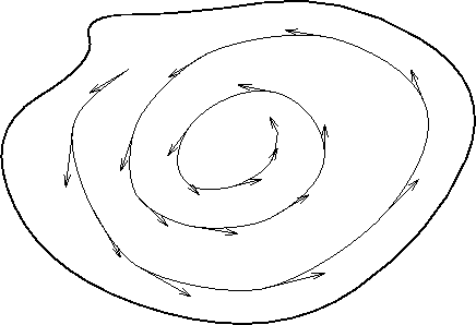
Given a vector field V we can apply the existence theorem for ordinary differential equations to construct a 1-parameter flow $\phi_{t}^{}$ on our space M. This satisfies $\phi_{t+s}^{}$ = $\phi_{t}^{}$o$\phi_{s}^{}$ and $\phi_{0}^{}$ fixes all points. Finally, we have d$\phi_{t}^{}$(p)/dt = V($\phi_{t}^{}$(p)); which is the ordinary differential equation we have solved. For any tensor field A, the following limit exists by differentiability of the quantities involved

L_V(A)(p) = $$\lim_{t\to 0}^{}$$$${\frac{A(p) - \phi_{-t} A(\phi_t(p))}{t}}$$

and it is called the Lie derivative of A with respect to V. For a pair of vector fields V and W it is not difficult to show that L_V(f )(p) = $\nabla_{V(p)}^{}$(f ) for any differentiable function f and

L_V(W)(p) = $$\nabla_{V(p)}^{}$$(W) - $$\nabla_{W(p)}^{}$$(V)

for any vector field W (and hence L_V(W) = - L_W(V)). Note that L_V(W) involves the derivatives of V even though the derivative is being taken (in some sense) with respect to V.

Figure 9: A tangent vector field and its flow

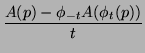
While the gradient of a function is independent of a choice of coordinates because of the interpretation as Lie derivative, the gradient of a tensor of order at least 1 is clearly dependent upon the choice of coordinates, thus it is natural to ask for a derivation D that is in some sense ``canonical''. This is provided by the condition that the inner product form < , > has no derivative,

D_{$\;\stackrel{\rightarrow}{u}\;$}( < V, W > ) = < D_{$\;\stackrel{\rightarrow}{u}\;$}(V), W > + < V, D_{$\;\stackrel{\rightarrow}{u}\;$}(W) >

where D_{$\;\stackrel{\rightarrow}{u}\;$}(f )= $\nabla_{\vec{u}}^{}$(f ) as before for any function f. In addition we demand the condition that the derivation is torsion-free,

L_V(W)(p) = D_V(p)(W) - D_W(p)(V)

This can be translated into the condition on the connection form $\omega$

$$\omega$$($$\;\stackrel{\rightarrow}{v}\;$$)($$\;\stackrel{\rightarrow}{w}\;$$) = $$\omega$$($$\;\stackrel{\rightarrow}{w}\;$$)($$\;\stackrel{\rightarrow}{v}\;$$)

There is then a unique such derivation and thus it is independent of any choice of coordinates.

In geometric terms, the usual gradient $\nabla_{\vec{v}}^{}$(A) measures the deviation of A(p + t$\;\stackrel{\rightarrow}{v}\;$) from a copy of A(p) moved to the point p + t$\;\stackrel{\rightarrow}{v}\;$. However, this motion requires a notion of parallel transport or rigid motion--which may be different for our geometry from the Euclidean one provided by the coordinates; the Riemannian metric provides the correct notion of angles and distances and hence of rigid motion. Thus D provides the ``corrected'' gradient.

Now it is conceivable that there is a choice of coordinates in which the $\omega$($\;\stackrel{\rightarrow}{v}\;$)'s vanish or simplify. Thus we need to find some way of checking this possibility. Riemann introduced the Riemannian curvature as a measure of this. This was modified by Christoffel who defined the curvature operator as follows. First of all for a vector field V and a tensor field A let us define D_V(A)(p) = D_V(p)(A). We then define the operator R by

R(V, W)(X) = D_V(D_W(X)) - D_W(D_V(X)) - D_LV(W)(X)

One checks that for any functions f, g and h we have

R(fV, gW)(hX) = fgh ^. R(V, W)(X)

From this it follows that for each point p, R(V, W) defines an endomorphism of the tangent space which depends only on the values V(p) and W(p). We can thus denote this by R($\;\stackrel{\rightarrow}{v}\;$,$\;\stackrel{\rightarrow}{w}\;$). The Riemannian curvature is then defined by

K($$\;\stackrel{\rightarrow}{v}\;$$,$$\;\stackrel{\rightarrow}{w}\;$$,$$\;\stackrel{\rightarrow}{x}\;$$,$$\;\stackrel{\rightarrow}{y}\;$$) = < R($$\;\stackrel{\rightarrow}{v}\;$$,$$\;\stackrel{\rightarrow}{w}\;$$)($$\;\stackrel{\rightarrow}{x}\;$$),$$\;\stackrel{\rightarrow}{y}\;$$ >

Bianchi proved that K($\;\stackrel{\rightarrow}{v}\;$,$\;\stackrel{\rightarrow}{w}\;$,$\;\stackrel{\rightarrow}{x}\;$,$\;\stackrel{\rightarrow}{y}\;$) = K($\;\stackrel{\rightarrow}{x}\;$,$\;\stackrel{\rightarrow}{y}\;$,$\;\stackrel{\rightarrow}{v}\;$,$\;\stackrel{\rightarrow}{w}\;$), and for any three vector fields U, V, W

(D_UR)(V, W) + (D_WR)(U, V) + (D_VR)(W, U) = 0

We now consider the curvature as a function of a pair of tensors of order 2

S($$\;\stackrel{\rightarrow}{v}\;$$ $$\otimes$$ $$\;\stackrel{\rightarrow}{w}\;$$,$$\;\stackrel{\rightarrow}{x}\;$$ $$\otimes$$ $$\;\stackrel{\rightarrow}{y}\;$$) = K($$\;\stackrel{\rightarrow}{v}\;$$,$$\;\stackrel{\rightarrow}{w}\;$$,$$\;\stackrel{\rightarrow}{x}\;$$,$$\;\stackrel{\rightarrow}{y}\;$$)

As usual we introduce the notation

$$\;\stackrel{\rightarrow}{v}\;$$ $$\wedge$$ $$\;\stackrel{\rightarrow}{w}\;$$ = $${\textstyle\frac{1}{2}}$$($$\;\stackrel{\rightarrow}{v}\;$$ $$\otimes$$ $$\;\stackrel{\rightarrow}{w}\;$$ - $$\;\stackrel{\rightarrow}{w}\;$$ $$\otimes$$ $$\;\stackrel{\rightarrow}{v}\;$$)

for skew-symmetric tensors of order 2. Then we have

S($$\;\stackrel{\rightarrow}{v}\;$$ $$\otimes$$ $$\;\stackrel{\rightarrow}{w}\;$$,$$\;\stackrel{\rightarrow}{x}\;$$ $$\otimes$$ $$\;\stackrel{\rightarrow}{y}\;$$) = S($$\;\stackrel{\rightarrow}{v}\;$$ $$\wedge$$ $$\;\stackrel{\rightarrow}{w}\;$$,$$\;\stackrel{\rightarrow}{x}\;$$ $$\wedge$$ $$\;\stackrel{\rightarrow}{y}\;$$)

Moreover S($\;\stackrel{\rightarrow}{v}\;$ $\wedge$ $\;\stackrel{\rightarrow}{w}\;$,$\;\stackrel{\rightarrow}{x}\;$ $\wedge$ $\;\stackrel{\rightarrow}{y}\;$) is a symmetric bilinear pairing on the space of skew-symmetric tensors of order 2. Now one such is given by the pairing of tensors

< $$\;\stackrel{\rightarrow}{v}\;$$ $$\wedge$$ $$\;\stackrel{\rightarrow}{w}\;$$,$$\;\stackrel{\rightarrow}{x}\;$$ $$\wedge$$ $$\;\stackrel{\rightarrow}{y}\;$$ > = $${\textstyle\frac{1}{2}}$$( < $$\;\stackrel{\rightarrow}{v}\;$$,$$\;\stackrel{\rightarrow}{x}\;$$ > < $$\;\stackrel{\rightarrow}{w}\;$$,$$\;\stackrel{\rightarrow}{y}\;$$ > - < $$\;\stackrel{\rightarrow}{v}\;$$,$$\;\stackrel{\rightarrow}{y}\;$$ > < $$\;\stackrel{\rightarrow}{w}\;$$,$$\;\stackrel{\rightarrow}{x}\;$$ > )

A comparison of the associated quadratic forms is then given by the ratio

$$\kappa$$($$\;\stackrel{\rightarrow}{v}\;$$,$$\;\stackrel{\rightarrow}{w}\;$$) = - $${\frac{K(\vec{v},\vec{w},\vec{v},\vec{w})}{%% <\vec{v},\vec{v}><\vec{w},\vec{w}> - <\vec{v},\vec{w}>^2}}$$

This is what is called the sectional curvature of the Riemannian manifold (the sign is for reasons of convention). This is by far the most important invariant associated with a Riemannian manifold. It is clear from the above discussion that the sectional curvature, the Riemannian curvature and the Riemann-Christoffel operator on a Riemannian manifold determine each other.

An important result of Cartan and Hadamard (see [3]) states that any Riemannian space M as above with the property that its sectional curvature is constant can be identified with an open subset of either the Euclidean space or Hyperbolic (Bolyai-Lobachevsky) space or Projective space in an isometric way.

We will see in the next section how to apply this to the study of axiomatic geometries.