8.2 Functors of points

Suppose that we are given a system S of p polynomial equations in q variables. To every finite ring A we associate the set S(A) of all q-tuples (a₁,..., a_q) of elements of A that satisfy this system of equations. This is an example of a functor F from finite rings to finite sets; i. e. for every ring A we associate a finite set F(A) such that if A$\to$B is a ring homomorphism then we have a natural map F(A)$\to$F(B) so that composition of ring homomorphisms goes to composition of set maps and the identity ring homomorphism goes to the identity map.

Giving a system T that is ``derived'' from the system S by substituting the variables by polynomial functions of another set of r variables is a natural operation on systems of equations. The analogous notion is that of a morphism of functors (also called a natural transformation) F$\to$G. This is a way of giving a map F(A)$\to$G(A) so that for any ring homomorphism A$\to$B we get a commutative diagram (any element in the top left corner has the same image in the bottom right corner independent of the route followed).

F(A)	$$\to$$	G(A)
$$\downarrow$$		$$\downarrow$$
F(B)	$$\to$$	G(B)

Some simple examples of such functors are:

1. To every finite ring we associate the empty set.
2. To every finite ring we associate the singleton set.
3. To every finite ring we associate the underlying set of the ring.
4. To every finite ring we associate the group of units in the ring.
5. To every finite ring we associate the collection of q tuples of elements of the ring.

Each of the above is a particular case of the following more general construction. Let R be any finitely generated ring (i. e. R is a the quotient of the ring $\mathbb {Z}$[X₁,..., X_q] of polynomials with integer coefficients by some ideal I). We have a functor (usually denoted by Spec(R)) which associates to the finite ring A the finite set of (unital) ring homomorphisms Hom(R, A). This can be done by taking the rings (1) R = 0 (2) R = $\mathbb {Z}$ (3) R = $\mathbb {Z}$[X] (4) R = $\mathbb {Z}$[X, Y]/(XY - 1) and (5) R = $\mathbb {Z}$[X_r..., X_q]. The associated geometric objects can conceptualised as (1) empty (2) point (3) line (4) hyperbola (5) q-dimensional affine space $\mathbb {A}$^q (since that is what one will get when A is a field). A functor of the form Spec(R) for a finitely generated ring R is called an affine scheme. If R is a quotient of the polynomial ring $\mathbb {Z}$[X₁,..., X_q] by the ideal generated by polynomials (f₁(X₁,..., X_q),..., f_p(X₁,..., X_q)), then it is clear that Spec(R)(A) is naturally identified with the subset of q-tuples of elements of A which satisfy the system of equations given by the f_i.

For those who have studied affine schemes earlier in a slightly different way we offer the following result which is proved in the second appendix.

Lemma 17   Let R$\to$S be a homomorphism of finitely generated rings so that for every finite ring A the induced map Hom(S, A)$\to$Hom(R, A) is a bijection. Then this homomorphism is an isomorphism.

A slightly different example (but one which is fundamental) is the functor that associates with a ring A the collection of all n + 1-tuples (a₀, a₁,..., a_n) which generate the ring A upto multiplication by units. Equivalently, one can think of all surjective A-module homomorphisms A^{n + 1}$\to$A modulo the equivalence induced by multiplication by units. This functor is denoted $\mathbb {P}$ⁿ and is conceptualised as the projective n-dimensional space. We use the symbol (a₀ : a₁ : ^... : a_n) to denote the equivalence class under unit multiples of the n + 1-tuple (a₀, d₁,..., a_n) which gives rise to an element in $\mathbb {P}$ⁿ(A).

Now, if a = (a₀ : a₁ : ^... : a_p) and b = (b₀ : b₁ : ^... : b_q) are elements in $\mathbb {P}$^p(A) and $\mathbb {P}$^q(A) respectively, then we can form the (p + 1) ^. (q + 1)-tuple consisting of c_ij = a_j ^. b_j; this tuple generates the ring A as well. Clearly, when a and b are replaced by unit multiples ua and vb for some units u and v in A, the tuple c = (c_ij)_{i = 0, j = 0}^{p, q} is replaced by its unit multiple (uv)c. Thus, we have a natural transformation $\mathbb {P}$^p×$\mathbb {P}$^q$\to$$\mathbb {P}$^{pq + p + q}. Moreover, one easily checks that the resulting map on sets

$$\mathbb {P}$$^p(A)×$$\mathbb {P}$$^q(A)$$\to$$$$\mathbb {P}$$^{pq + p + q}(A)

is on-to-one for every finite ring A. This natural transformation is called the Segre embedding.

For each positive integer d we can associate to a = (a₀ : a₁ : ^... : a_p) the $\binom{p+d}{d}$ tuple of all monomials of degree exactly d with the entries from a. For example, if d = 2 then we take the $\binom{p+2}{2}$-tuple consisting of b_ij = a_ia_j. As above this gives a natural transformation of functors $\mathbb {P}$^p$\to$$\mathbb {P}$^{$\binom{p+d}{d}$ - 1}. For each finite ring A the resulting map on sets

$$\mathbb {P}$$^p(A)$$\to$$$$\mathbb {P}$$^{$\binom{p+d}{d}$ - 1}(A)

is one-to-one. This natural transformation is called the d-tuple Veronese embedding.

The two examples above are special cases of projective subschemes defined as follows. Let F(X₀,..., X_p) be any homogeneous polynomial in the variables X₀,...,X_p (in other words all the monomials in F have the same degree). While the value of F at a p + 1-tuple (a₀,..., a_p) can change if we multiply the latter by a unit, this multiplication does nothing if the value is 0. Thus, the set

V(F)(A) = {(a₀ : a₁ : ^... : a_p)| F(a₀,..., a_p) = 0}

is well-defined. More generally, we can define, for any finite collection F₁,..., F_n of homogeneous polynomials in the same p + 1 variables

V(F₁,..., F_n)(A) = {(a₀ : a₁ : ^... : a_p)| F_i(a₀,..., a_p) = 0;$$\forall$$i}

Such sub-functors of $\mathbb {P}$^p(A) are called projective schemes. To emphasise the point, a functor is a projective scheme if it is naturally isomorphic to one of the functors of the form V(F₁,..., F_n) for some homogeneous polynomials F_i in the set of p + 1 variables X_i. In particular, the Segre embedding is given by the system of all equations of the form Z_ijZ_kl = Z_ilZ_kj. For any monomial of degree 2d and two ways of writing it as a product of monomials of degree d, we obtain a quadratic equation satisfied by the elements of the Veronese embedding; this system of equations defines the Veronese embedding.

There is also a natural way of thinking of affine schemes in terms of subfunctors of $\mathbb {P}$ⁿ for a suitable n. As we saw above any affine scheme is a subscheme of $\mathbb {A}$^q, so it is enough to exhibit $\mathbb {A}$^q as a subfunctor of $\mathbb {P}$ⁿ for a suitable n. Now it is clear that if (a₁,..., a_q) is any q-tuple, then the collection (1, a₁,..., a_q) generates the ring A so that this defines an element (1 : a₁ : ^... : a_q) of $\mathbb {P}$^q(A). Conversely, if (a₀ : a₁ : ^... : a_q) is an element of $\mathbb {P}$^q(A), such that a₀ is a unit then this is the same as (1 : a₁/a₀ : ^... : a_q/a₀), which in turn corresponds to the point (a₁/a₀,..., a_q/a₀) in $\mathbb {A}$^q.

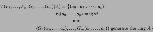
A generalisation of the above is the notion of a quasi-projective scheme. In addition to the homogeneous polynomials F_i considered above let G₁(X₀,..., X_p), ..., G_m(X₀,..., X_p) be homogeneous polynomials of the same degree. We define a quasi-projective scheme

$$\begin{multline*} V(F_1,\dots,F_n;G_1,\dots,G_m)(A) = \left\{ \strut (a_0:a_1:... ...dots,G_m(a_0,\dots,a_p)) \text{ generate the ring } A \right\} \end{multline*}$$

Note that, we need to make sense of linear combinations of the G_i's and hence it is essential that they are all of the same degree. As before we will be interested in the underlying functor rather than its given representation as a subfunctor defined by the ``equations'' F<sub>i</sub> and the ``inequations'' G_j.

One can go further and define the notion of an abstract algebraic scheme but for our purposes the notion defined above of a quasi-projective scheme (of finite type over integers or of ``arithmetic'' type) will suffice.

Let F₁,...,F_n be a collection of equations which define a projective scheme and d be no smaller than the maximum of their degrees. It is clear that the same projective scheme is defined by the larger collection of the form F_j ^. M where j varies between 1 and n and M varies over all monomials of degree d - deg(F_j). Thus we can always assume that a projective scheme is defined by homogeneous equations of the same degree.

The complement of the subscheme of V(F₁,..., F_n) is not the functor that assigns to each A the set-theoretic complement $\mathbb {P}$^p(A) $\setminus$ V(F₁,..., F_n)(A), but in fact, when F_i's have the same degree it is the quasi-projective scheme V(0;F₁,..., F_n)(A). The reason for this choice becomes clear as we study schemes more. For the moment it is enough to note that if A is the ring $\mathbb {F}$_p[$\epsilon$] = $\mathbb {F}$_p[X]/(X²), then the element (1 : $\epsilon$ : ^... : $\epsilon$) is in the set-theoretic complement of (1 : 0 : ^... : 0) in $\mathbb {P}$^p(A) but is not in the scheme-theoretic complement that we have defined above.

Finally, let X $\subset$ $\mathbb {P}$^p be a quasi-projective scheme, and let F₁,..., F_n be a bunch of homogeneous polynomials of the same degree. The intersection X $\cap$ V(F₁,..., F_n;1) is clearly a subscheme of X and such subschemes are called closed subschemes of X. The intersection X $\cap$ V(0;F₁,..., F_n) is also a subscheme of X and such subschemes are called open subschemes of X. More generally, the intersection of V(D₁,..., D_m;E₁,..., E_n) and V(F₁,..., F_k;G₁,..., G_l) is the scheme

V(D₁,..., D_m, F₁,..., F_k;{E_i ^. G_j})

The ``Hilbert Basis theorem'' asserts that the intersection of any (not necessarily finite) collection of closed subschemes is a closed subscheme.

One very useful example of a closed subscheme is the subscheme $\mathbb {P}$^p $\subset$ $\mathbb {P}$^p×$\mathbb {P}$^p, which is the diagonal; this is a closed subscheme of the scheme $\mathbb {P}$^p×$\mathbb {P}$^p defined by the conditions X_iY_j = X_jY_i for 0 $\leq$ i, j $\leq$ p. For any p < q we can exhibit $\mathbb {P}$^p as the closed subscheme of $\mathbb {P}$^q given by X_i = 0 for p < i $\leq$ q.

Like the case of set-theoretic complement, the set-theoretic union of closed subschemes is in general not a closed subschemes. For example the smallest closed subscheme of $\mathbb {P}$² that contains L = V(X₁) and M = V(X₂) is easily seen to be V(X₁X₂); but it is possible for the product of two elements of a finite ring to be 0 without either of them being zero. Thus we can define the scheme-theoretic union of a collection of closed subschemes to be the smallest closed subscheme that contains the set-theoretic union (the set-theoretic union defines a subfunctor); such a scheme exists by Hilbert's basis theorem. From now on when we use the term union of schemes we shall always mean the scheme theoretic union.

A closed subscheme Y $\subset$ X is said to be a proper closed subscheme if for some finite ring A, the subset Y(A) $\subset$ X(A) is a proper subset. A scheme is said to be reducible if it can be written as the union of two distinct (but not necessarily disjoint!) proper closed subschemes. For example V(X₁X₂) in $\mathbb {P}$²) is the union of the two lines V(X₁) and V(X₂). Now even a proper closed subscheme Y $\subset$ X can be ``essentially'' all of X; for example consider the closed subscheme Y = V(X₂²) of the scheme X = V(X₂³). For any finite field F, we have Y(F) = X(F). A scheme X is said to be reduced if it has no proper closed subscheme Y such that Y(F) = X(F) for all finite fields F. Note that the scheme V(X₁X₂) is reduced but not irreducible, while V(X₁²) is irreducible but not reduced. Hilbert's Basis theorem can also be used to show that any scheme X has a closed subscheme Y so that Y is reduced and Y(F) = X(F) for finite fields F. As a consequence of the Lasker-Noether Primary Decomposition theorem any scheme can be written as the union of a finite collection of irreducible closed subschemes; moreover, the underlying reduced schemes of these closed subschemes are uniquely determined. For example, consider the scheme L = V(X₁², X₁X₂) in $\mathbb {P}$². One can show that that L is the union of the closed subschemes M = V(X₁) and N = V(X₁², X₁X₂, X₂²). But L can also be written as the union of M and K = V(X₁², X₀X₂, X₁X₂, X₂²); moreover N and K are distinct schemes.